
Imagine sailing down a river in a small motorboat on a weekend afternoon; the water is smooth, and you are enjoying the sunshine and cool breeze when suddenly you are hit in the head by a 20-pound silver carp. This is a risk now on many rivers and canal systems in Illinois and Missouri because of Asian carp. This fish—a group of species including the silver, black, grass, and big-head carp—has been farmed and eaten in China for over 1,000 years. It is one of the most important aquaculture food resources worldwide. In the United States, however, Asian carp is considered a dangerous invasive species that disrupt ecological community structure to threaten native species. The effects of invasive species (such as the Asian carp, kudzu vine, predatory snakehead fish, and zebra mussel) are just one aspect of what ecologists study to understand how populations interact within ecological communities and what impact natural and human-induced disturbances have on the characteristics of communities.
Populations are dynamic entities. Their size and composition fluctuate due to numerous factors, including seasonal and yearly environmental changes, natural disasters such as forest fires and volcanic eruptions, and competition for resources between and within species. The study of populations is called demography.
Population Size and Density
Populations are characterized by population size (total number of individuals) and population density (number of individuals per unit area). A population may have a large number of individuals that are distributed densely or sparsely. There are also populations with small numbers of individuals that may be dense or very sparsely distributed in a local area. Population size can affect the potential for adaptation because it affects the amount of genetic variation present in the population. Density can affect interactions within a population, such as competition for food and the ability of individuals to find a mate. Smaller organisms are more densely distributed than larger ones (Figure 1).
Estimating Population Size
The most accurate way to determine population size is to count all individuals within the area. However, this method is usually not logistically or economically feasible, especially when studying large areas. Thus, scientists usually study populations by sampling a representative portion of each habitat and use this sample to make inferences about the population as a whole. The methods used to sample populations to determine their size and density are typically tailored to the characteristics of the organism being studied. A quadrat may be used for immobile organisms such as plants or very small and slow-moving organisms. A quadrat is a square structure that is randomly located on the ground and used to count the number of individuals that lie within its boundaries. To obtain an accurate count using this method, the square must be placed at random locations within the habitat enough times to produce an accurate estimate.
For smaller mobile organisms, such as mammals, a technique called mark and recapture is often used. This method involves marking captured animals and releasing them back into the environment to mix with the rest of the population. Later, a new sample is captured, and scientists determine how many marked animals are in the new sample. This method assumes that the larger the population, the lower the percentage of marked organisms that will be recaptured since they will have mixed with more unmarked individuals. For example, if 80 field mice are captured, marked, and released into the forest, then a second trapping 100 field mice are captured, and 20 of them are marked, the population size (N) can be determined using the following equation:
N = (number marked first catch x total number of second catch)/number marked second catch
Using our example, the equation would be:
(80 x 100) / 20 = 400
These results give us an estimate of 400 total individuals in the original population. The true number usually will be a bit different from this because of chance errors and possible bias caused by the sampling methods.
Species Distribution
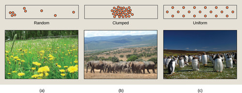
In addition to measuring size and density, further information about a population can be obtained by looking at the distribution of the individuals throughout their range. A species distribution pattern is the distribution of individuals within a habitat at a particular time—broad categories of patterns are used to describe them.
Individuals within a population can be distributed randomly, in groups, or equally spaced apart (more or less). These are known as random, clumped, and uniform distribution patterns (Figure 2). Different distributions reflect important aspects of the biology of the species. They also affect the mathematical methods required to estimate population sizes. An example of random distribution occurs with dandelion and other plants with wind-dispersed seeds germinating wherever they fall in favorable environments. A clumped distribution may be seen in plants that drop their seeds straight to the ground, such as oak trees; it can also be seen in animals that live in social groups (schools of fish or herds of elephants). Uniform distribution is observed in plants that secrete substances inhibiting the growth of nearby individuals (such as the release of toxic chemicals by sage plants). It is also seen in territorial animal species, such as penguins, that maintain a defined territory for nesting. Each individual’s territorial defensive behaviors create a regular distribution pattern of similar-sized territories and individuals within those territories. Thus, the distribution of the individuals within a population provides more information about how they interact with each other than a simple density measurement. Just as lower-density species might have more difficulty finding a mate, solitary species with a random distribution might have a similar difficulty when compared to social species clumped together in groups.
Life tables provide important information about the life history of an organism and the life expectancy of individuals at each age. They are modeled after actuarial tables used by the insurance industry for estimating human life expectancy. Life tables may include the probability of each age group dying before their next birthday, the percentage of surviving individuals dying at a particular age interval, their mortality rate, and their life expectancy at each interval. An example of a life table is shown in Table 1 from a study of Dall mountain sheep, a species native to northwestern North America. Notice that the population is divided into age intervals (column A).
As can be seen from the mortality rate data (column D), a high death rate occurred when the sheep were between six months and a year old and then increased even more from 8 to 12 years old, after which there were few survivors. The data indicate that if a sheep in this population survived to age one, it could be expected to live another 7.7 years on average, as shown by the life-expectancy numbers in column E.
| Life Table of Dall Mountain Sheep1 | ||||
|---|---|---|---|---|
| Age interval (years) | Number dying in age interval out of 1000 born | Number surviving at beginning of age interval out of 1000 born | Mortality rate per 1000 alive at beginning of age interval | Life expectancy or mean lifetime remaining to those attaining age interval |
| 0–0.5 | 54 | 1000 | 54.0 | 7.06 |
| 0.5–1 | 145 | 946 | 153.3 | — |
| 1–2 | 12 | 801 | 15.0 | 7.7 |
| 2–3 | 13 | 789 | 16.5 | 6.8 |
| 3–4 | 12 | 776 | 15.5 | 5.9 |
| 4–5 | 30 | 764 | 39.3 | 5.0 |
| 5–6 | 46 | 734 | 62.7 | 4.2 |
| 6–7 | 48 | 688 | 69.8 | 3.4 |
| 7–8 | 69 | 640 | 107.8 | 2.6 |
| 8–9 | 132 | 571 | 231.2 | 1.9 |
| 9–10 | 187 | 439 | 426.0 | 1.3 |
| 10–11 | 156 | 252 | 619.0 | 0.9 |
| 11–12 | 90 | 96 | 937.5 | 0.6 |
| 12–13 | 3 | 6 | 500.0 | 1.2 |
| 13–14 | 3 | 3 | 1000 | 0.7 |
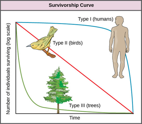
Another tool population ecologists use is a survivorship curve, a graph of the number of individuals surviving at each age interval versus time. These curves allow us to compare the life histories of different populations (Figure 3). There are three types of survivorship curves. In a type I curve, mortality is low in the early and middle years and occurs mostly in older individuals. Organisms exhibiting a type I survivorship typically produce few offspring and provide good care to the offspring, increasing their likelihood of survival. Humans and most mammals exhibit a type I survivorship curve. In type II curves, mortality is relatively constant throughout the entire lifespan, and mortality is equally likely to occur at any point in the life span. Many bird populations provide examples of an intermediate or type II survivorship curve. In type III survivorship curves, early ages experience the highest mortality with much lower mortality rates for organisms that make it to advanced years. Type III organisms typically produce large numbers of offspring but provide very little or no care for them. Trees and marine invertebrates exhibit a type III survivorship curve because very few of these organisms survive their younger years. Still, those that do make it to old age are more likely to survive for a relatively long period of time.
