
1 Revenue Management
Competencies
- Describe maximum revenue using derivatives of the revenue function for maximization.
- Use graphs to describe three key concepts of Revenue Management: revenue, supply, and demand.
- Outline why American Airlines started Revenue Management in graph illustration.
- Understand the 3 conditions for best use of Revenue Management: (1) High Fixed Cost and low Variable cost, (2) Fixed capacity and perishable products, and (3) Controllable demand.
Chapter 1 Outline
Derivatives of Revenue Function
- Derivatives of Revenue Function
- Supply curve as marginal cost
- Demand curve as utility cost
- Characteristics of business when applying Revenue Management
- Optimal price between supply and demand
- Industry applying Revenue Management
Revenue management, often called the art of “selling the right product to the right customer at the right time for the right price,” integrates data analytics, demand forecasting, and pricing strategies to optimize financial performance. It originated in the airline industry but has since expanded to hospitality, retail, and car rental sectors.
Pioneered by American Airlines in the 1980s, revenue management’s core principles involve understanding customer behavior, segmenting markets, and dynamically adjusting prices based on real-time data and predictive analytics. The seminal work by Robert G. Cross, “Revenue Management: Hard-Core Tactics for Market Domination” (1997) (1), remains a cornerstone reference, illustrating the transformative impact of these strategies on profitability and competitive advantage.
This chapter applies linear algebra graphs to describe key revenue management concepts and analyze the constraint conditions in the hospitality industry.
1. Derivatives of Revenue Function
Derivatives in linear algebra play a critical role in maximizing revenue and minimizing costs. The hotel’s goal is an objective function F(xi), where xi represents the variables influencing revenue and cost (e.g., room rates, occupancy rates, wages). Hotels operate under various constraints such as room availability, budget limits, or market demand. These constraints can be expressed as linear equations or inequalities, forming a feasible region where the solution must lie. Linear programming is a method used to achieve the best outcome in a mathematical model with linear relationships. The objective function and constraints are linear, and the solution involves finding the maximum or minimum value of the objective function within the feasible region. The partial derivatives under the gradient vector provide the direction of the steepest ascent or descent. In optimization, the gradient vector helps in understanding how changes in the variables affect the objective function. Directional derivatives provide insights into how the objective function changes as we move in a specific direction within the feasible region. When dealing with constraints, Lagrange multipliers are used to find the local maxima and minima of a function subject to equality constraints. The method involves introducing auxiliary variables (Lagrange multipliers) for each constraint and forming a Lagrangian function. To find the optimal solution, we take the partial derivatives of the Lagrangian function concerning the variables. The Lamda index of Lagrange multipliers indicates the magnitude of revenue maximization or cost minimization by changing the units of variables.
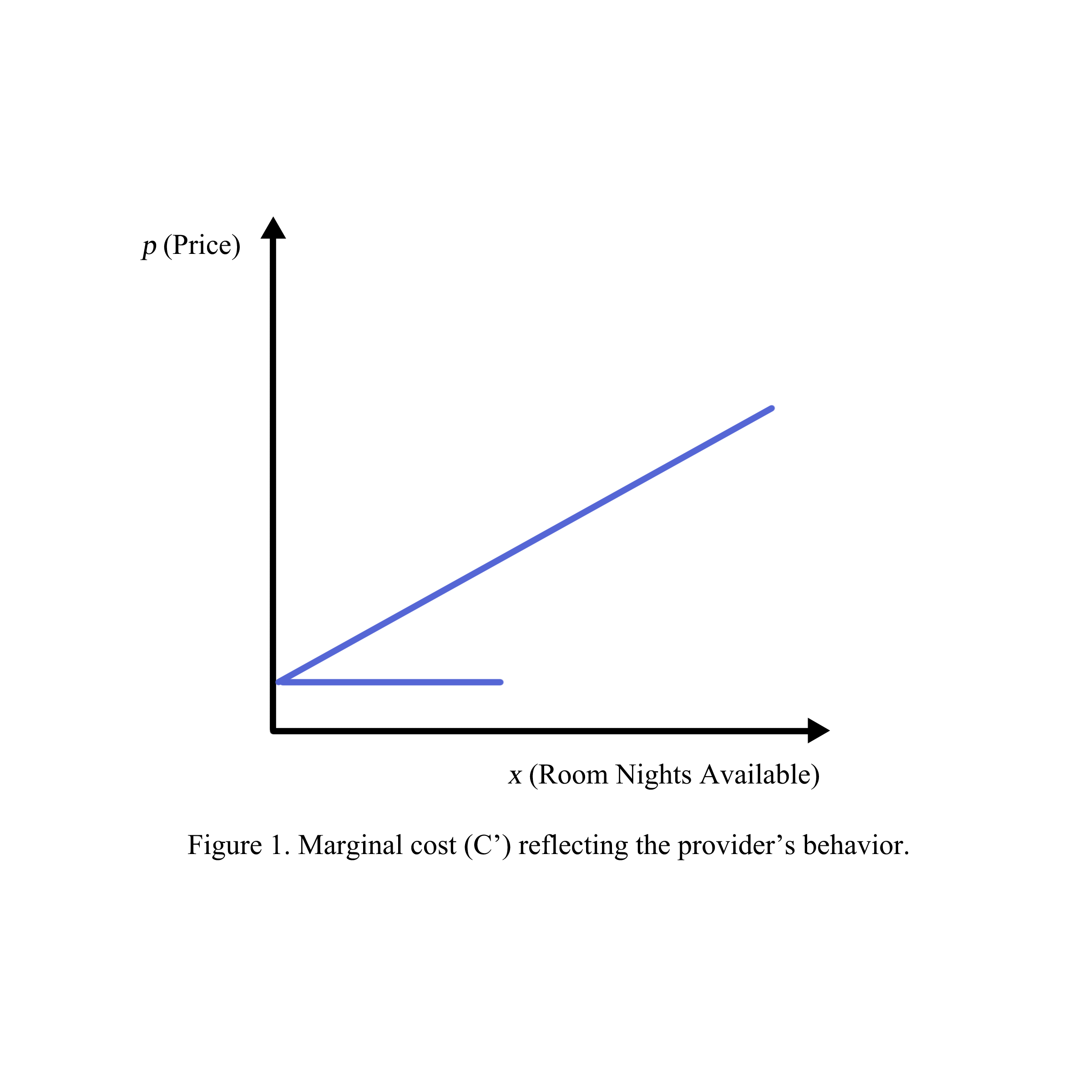
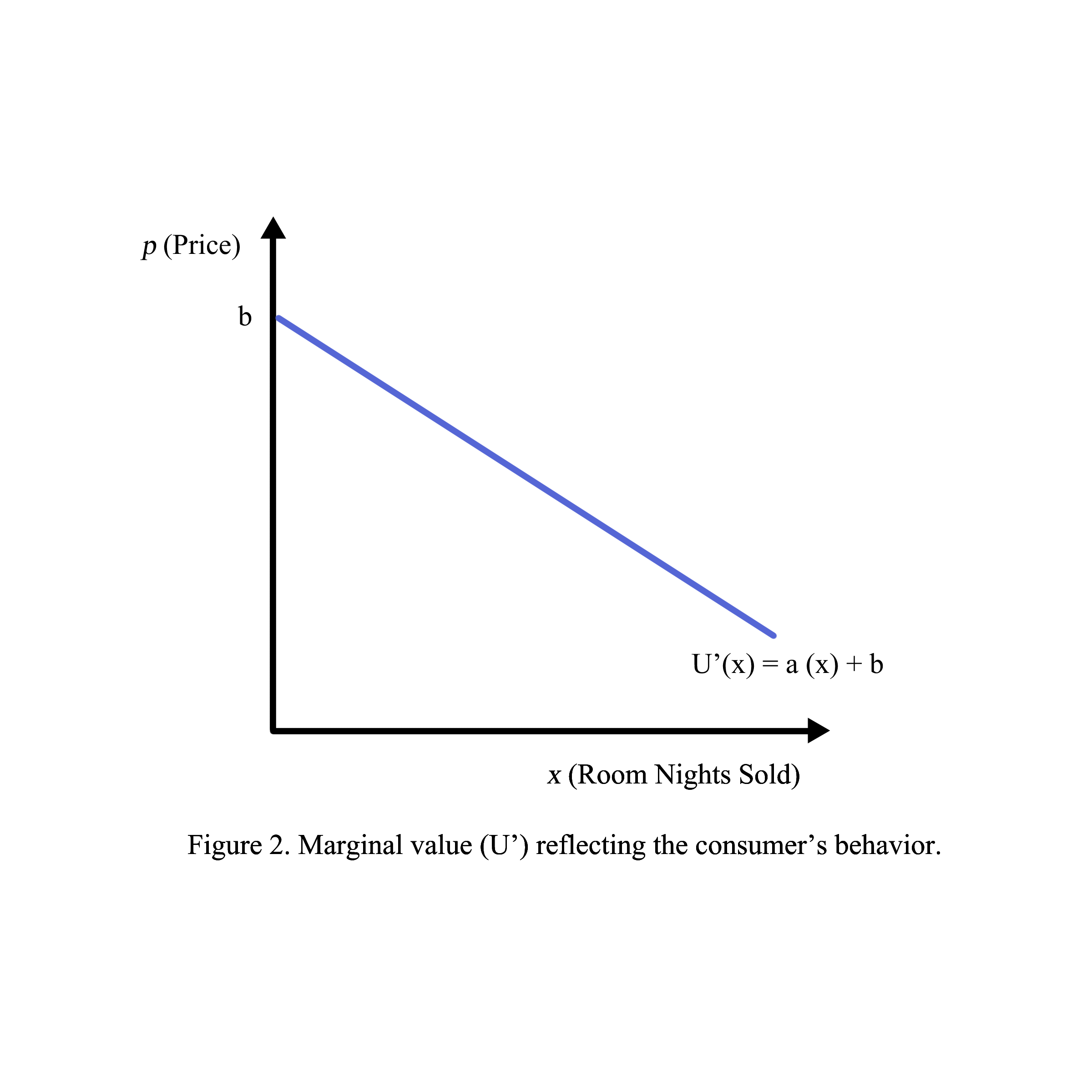
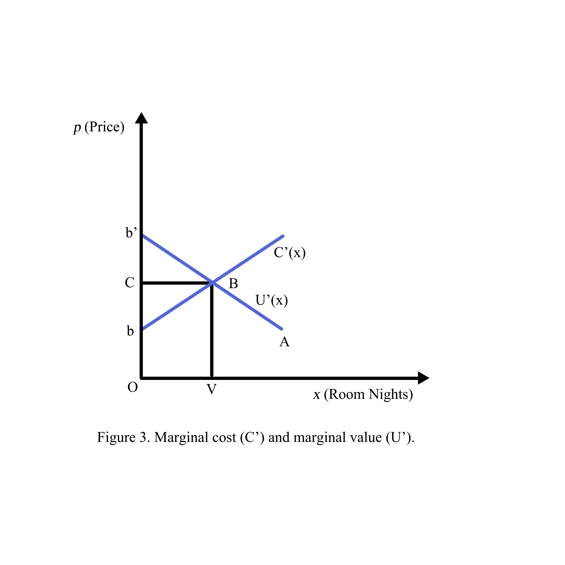
In this book, the derivative of cost (C) denoted by C’ called marginal cost reflects the provider’s price which is the steepest ascent since an additional room night built will increase the costs and room rates (figure 1). In contrast, the derivative of utility reflects the guest’s satisfaction which is the steepest descent (figure 2) since an additional room night will make the guest feel less excited than the beginning day at the hotel. The two derivatives U’ and C’ reflect the maximum of U and minimum of cost (figure 3). The derivatives of cost and utility are analyzed in breakeven with a minimum price to get profit (figure 4), a substitute compensated effect in potential maximum average daily rate (figure 5), a price elasticity of demand through the ratio between two derivatives of price and number of room nights (figure 6), matching the derivatives of the satisfaction of group or transient (figure 7), matching the derivatives of distribution channels (figure 8), matching the derivatives of guest income (figure 9), matching the derivatives of seasonality by derivatives through time series (figure 10), and finally matching the maximum of revenue by maximize revenue function through Lagrange lambda in partial derivatives of the constraints of budget and income (figure 11).
Revenue management is comprised of strategies of the provider to appeal most the consumer to maximize the revenue for his business. Revenue management is also called yield management because the producer’s attempts to forecast the consumer’s demand have yielded his aspiration to understand the consumer first. There are 2 key characters in the market: the producer and the consumer, whose behaviors are reflected in the marginal cost for the producer and the marginal utility for the consumer. The relationships among them are analyzed as follows:
1.1. The producer produces a service/product in the model: y= ax + b where:
y: unit price; e.g., the rate of one room per night in the hotel including a fixed cost, a variable cost, and a profit,
x: number of units for sale; in the hotel, it is the number of room nights available in a hotel called hotel supply,
a: marginal cost of one additional unit; in the hotel, the marginal cost is the cost of additional one room night for sale,
b: the fixed cost distributed in the unit price
For example, when the producer sells one more room per night, the marginal cost is C‘ in which a is the variable cost of cleaning and b is the fixed cost depreciated for one room per night (Figure 1).
1.2. The consumer pays for the producer’s service/product in the model U=-ax+b where:
U: the unit price sold or the average daily rate for a hotel, x: number of units sold; the number of room nights sold called hotel demand,
a: marginal utility of the consumer; since the consumer wants to pay less for an additional one, the value of a’ is negative for one room night purchased; it is negative due to the consumer’s willingness to pay less,
b: the maximum amount of payment the consumer is willing to pay for the unit service/product; e.g., the potential average daily rate in the hotel
Figure 2 indicates when a guest purchased one room per night, his payment would be U‘ in which a is the room rate for an additional night and b is the potential average daily rate.
1.3. The consumer and producer relationship is significant at two points: B where marginal cost meets marginal utility and A where marginal utility is zero. At point B, the producer and the consumer are both happy due to their benefit equality (b’BC=CBb). At the “happy time”, the revenue of the producer may not be the maximum revenue since the price point to maximize revenue is Ob’ where the marginal revenue b’b met the marginal cost C’(x) called potential ADR. The unit price OC will be ADR and RevPAR because of 100% occupancy when supply=demand=OD. At point A, the producer and the consumer will not exchange anything since the consumer stops buying and the producer stops selling (Figure 3).
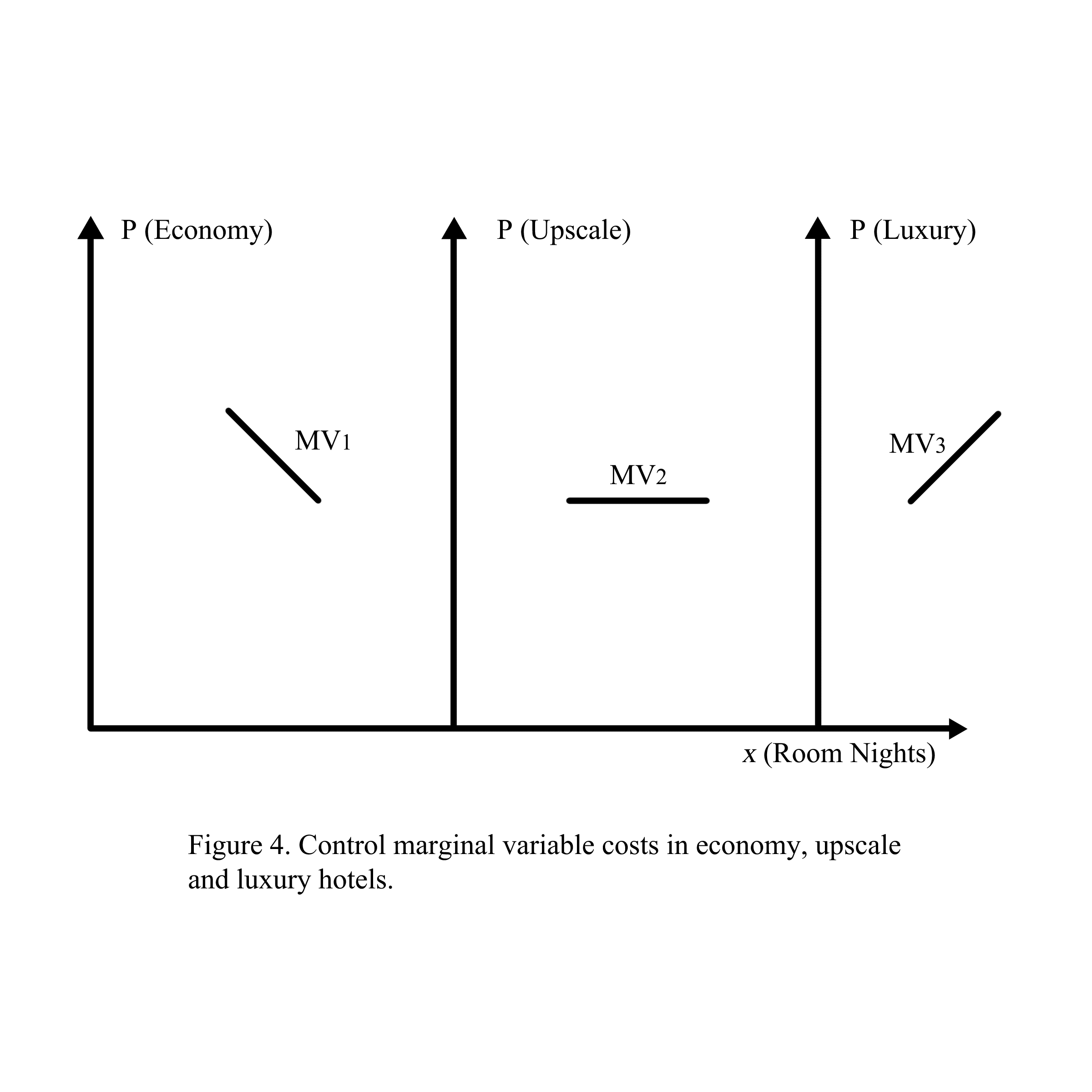
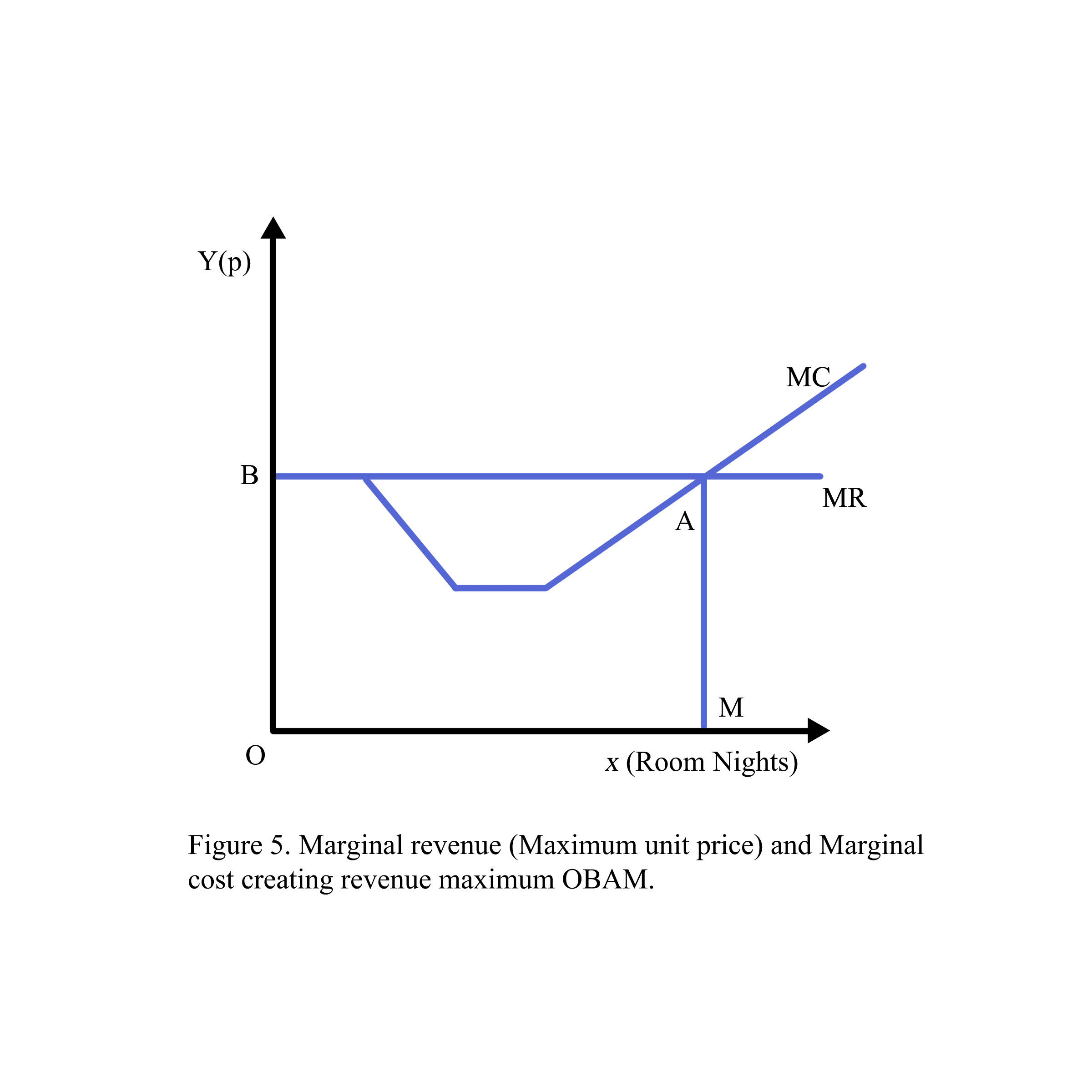
Revenue management is a collection of strategies to maximize revenue for the producer based on the willingness-to-pay of the consumer. The process to maximize the revenue of the producer starts from controlling costs (Figure 4) and competing with other competitors (Figure 5) to forecasting consumer demand (Figure 6), manipulation (Figure 7), and distributing the products/services to the consumer (Figure 8).
1.3.1. Controlling cost
To maximize revenue, the producer must first control cost through the constant marginal cost in the competitive bench-marking as follows:
TC(x) = FC + VC(x) (1)
Where
TC: Total cost
FC: Fixed cost
VC: Variable cost
x: The number of units for sale (number of hotel room nights available). If the cleaning room which is the key part of the variable cost is controlled as a constant, the marginal cost will be measured in Figure 4 as follows
Marginal cost = (TC(x))’ = FC + (VC(x))’ = FC + 0
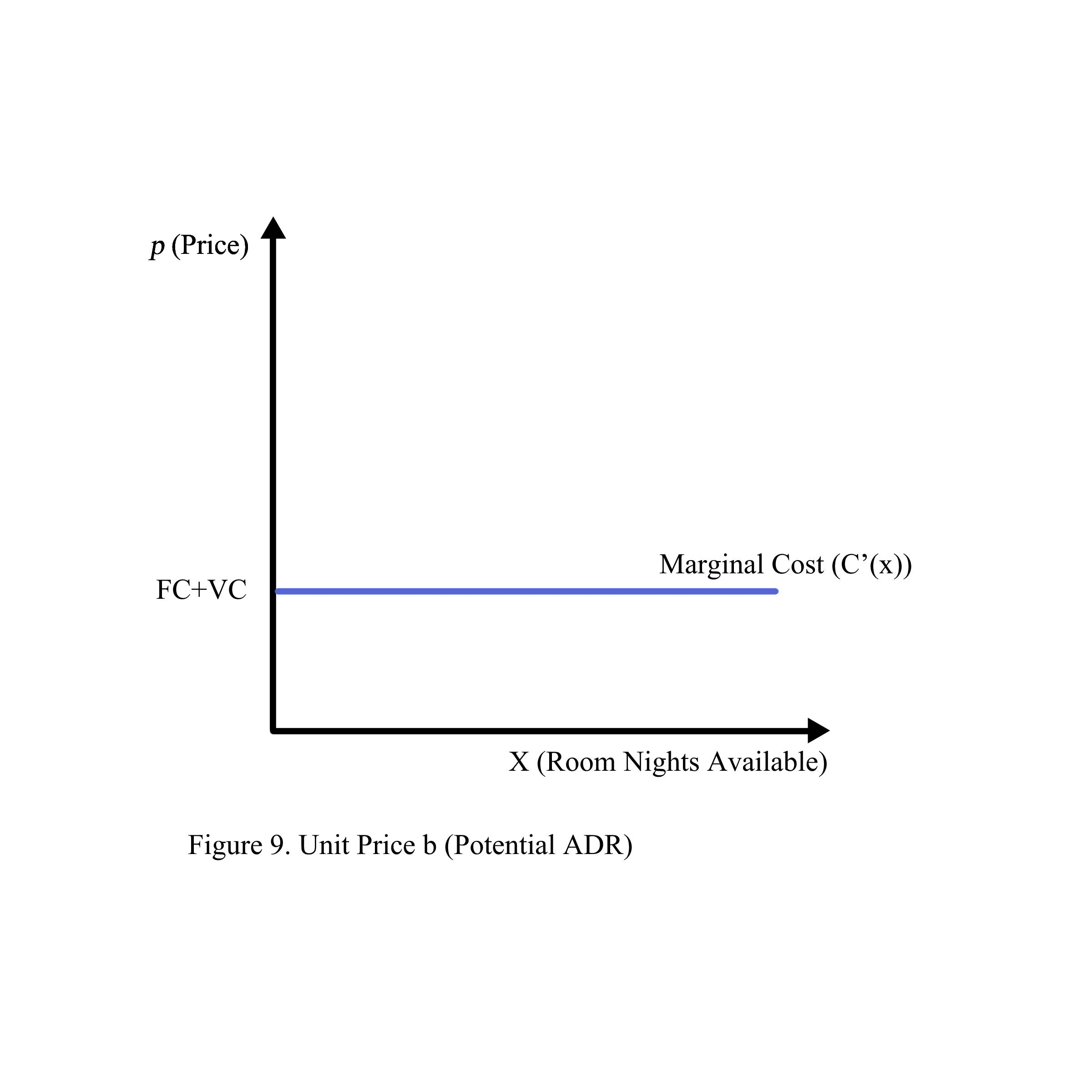
1.3.2. Setting potential unit price (the maximum price the consumer may be willing to pay for a unit product/service) (Figure 5)
After keeping the marginal cost constant, the producer will set the potential unit price b which is the maximum price the consumer could pay as follows:
b = Potential unit price (Potential ADR) = FC + VC + MP
Where: FC: Fixed cost, VC: Variable Cost, and MP: Maximized Profit
1.3.3. Forecasting consumer demand
After setting the maximum price, forecasting consumer demand is the next step to measure the responsiveness of the consumer when he consumes an additional product/service. The consumer is forecasted to maximize his benefits, that is:
Consumer benefit = Total value of consumption – (Price * Quantity) = u(x)-p*x
Where x: the number of consumed units
U(x) is a function describing the value of the consumed product/service (or utility)
The consumer benefit is maximized when its derivative equals zero, that is,
U’(x) – p = 0
U’(x) = p
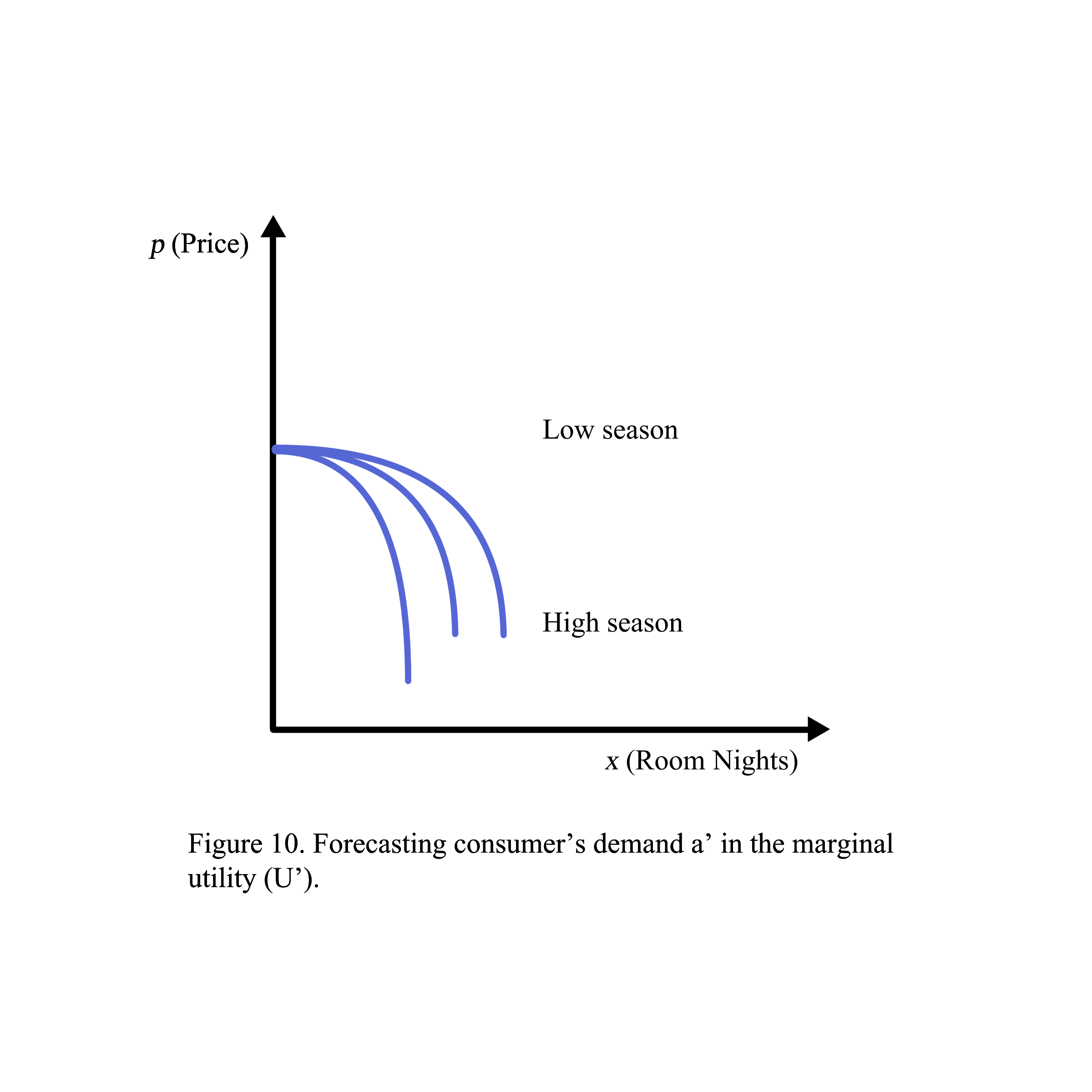
Based on the law of diminishing marginal utility, when the consumer wants more, his marginal utility will decline. The marginal utility is described as linear as follows:
U’(x) = b – a’x
where:
U’: marginal utility
b: maximized price the consumer pays for one unit (potential ADR)
a’: level of decline per additional consumed unit
x: number of consumed units (Figure 6).
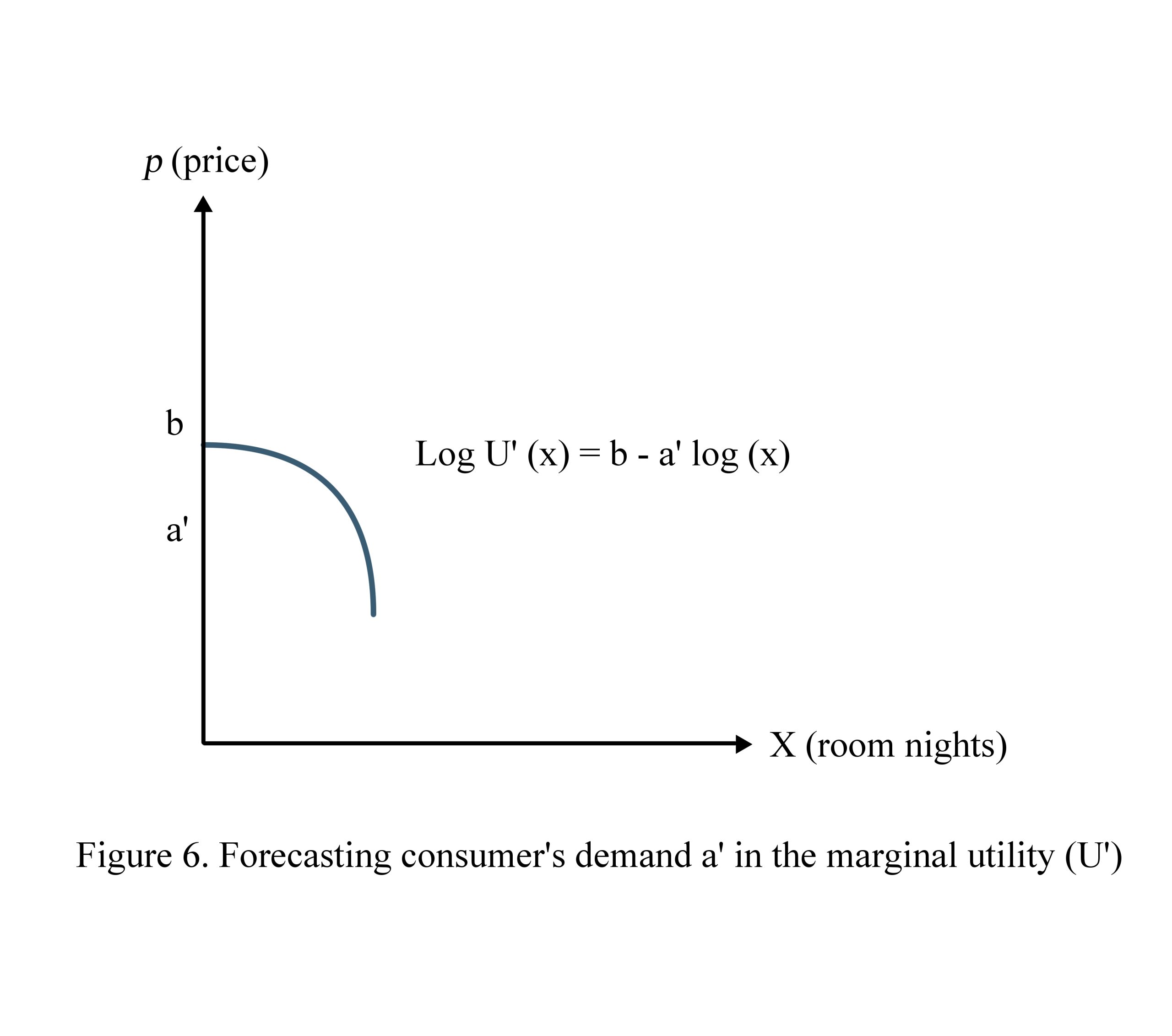
Forecasting consumer demand is forecasting the level of declining a’. The smaller the value a’ is, the steeper the U’ becomes. Elasticity is a tool to measure the steeper responsiveness of the consumer.
In practice, the log function replaces the linear for more precision in forecasting. The slope a’ is then measured by
(Difference in Quantity/Quantity) / (Difference in Price/Price)
1.3.4. Manipulation
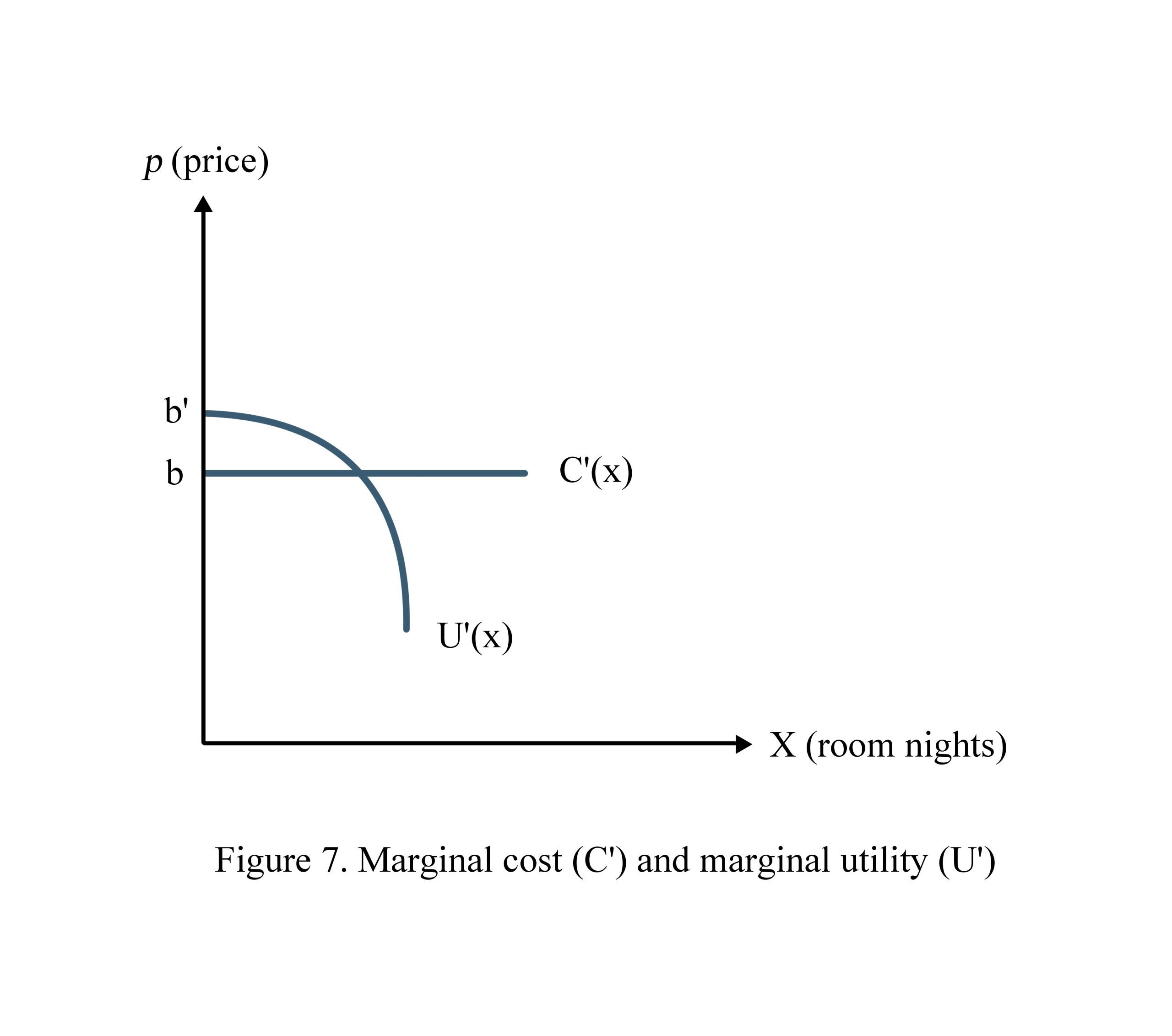
After forecasting demand, the producer will change the potential price at the beginning to fit the price elasticity of demand (PED) in Figure 7 as follows:
1.3.5. Distribution
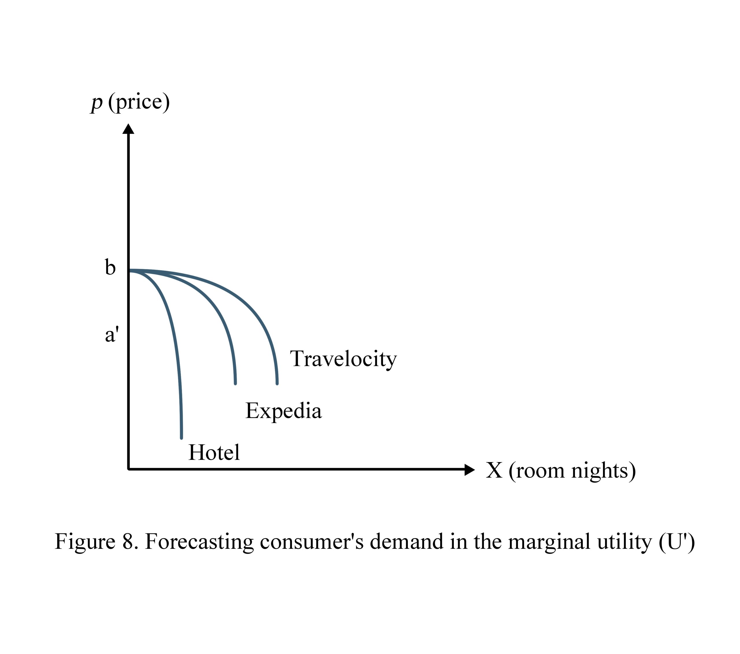
After resetting the potential ADR, the hotelier will set the distribution channels that match the value of a’ in Figure 8 as follows:
1.4. Characteristics of business when applying Revenue Management
There are two main characteristics of the business that need revenue management
1.4.1. High Fixed Low Variables (Figure 9)
The fixed cost is the absolute cost for all the supplies, building costs, land, etc. The variable cost includes the wages to hire workers, housekeepers, etc.
1.4.2. Seasonal products/services (Figure 10)
The hotel business is called seasonal products/services. High seasonal products in May, June, July, or August are an approximated time when customers are most common/checking in most often. These seasonal times are best for increasing supplies to keep up with demand. The service part is that when possible, employees come in for employment.
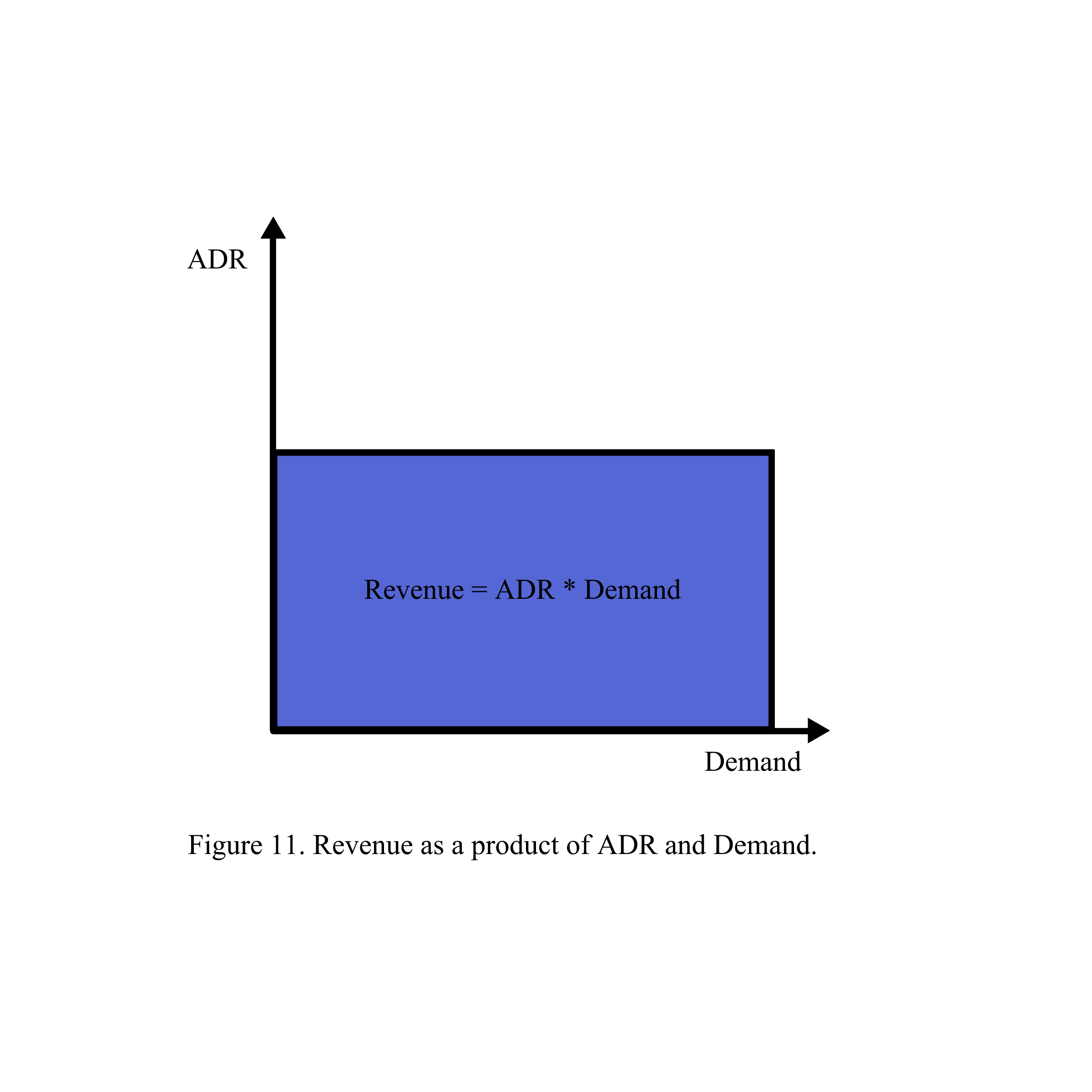
1.5. Revenue
Revenue management is a technique to maximize revenue through changing supply and demand. Revenue of hotel rooms is all payments received from the hotel guests staying at the hotel rooms during a period. Revenue is measured by the number of room nights the guests stayed (demand) multiplied by the room-night rate; hotel average daily rate (ADR) illustrated in Figure 11.
2. Supply curve as marginal cost
Supply is the quantity the producer can provide to the consumer. Hotel room supply is the number of room nights available a hotel is able to provide for hotel guests. To reach the maximum of revenue, a hotel needs to have the optimal number of room nights available (s1), not the maximum number of supply (S). The optimal supply s1 can be measured by marginal cost calculated as follows:
Profit = Price*Quantity – Cost
P(s) = ps – C(s)
Where P(s) is profit of the hotel room services; p is the rate of one room per night (Average daily rate); s is the number of room nights available and C is the direct expenses for one room per night.
In a hotel, when s is equal to the number of room nights available and s1 maximizes the profit P(x), the derivative of the function must be set to zero. That is, the hotel’s maximum profit occurs when
P’(s) = p – C’(s) = 0 (Figure 12)
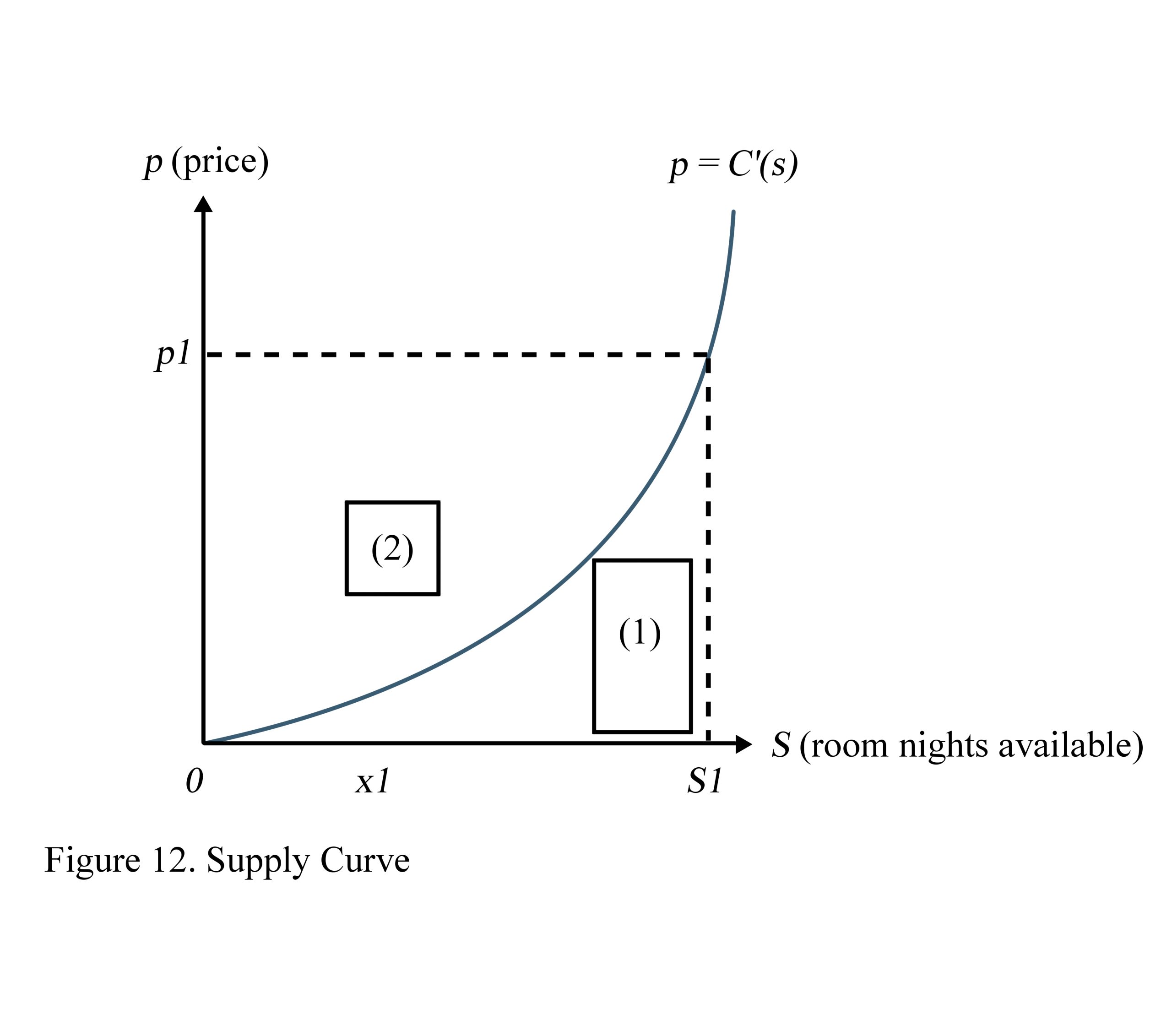
Price p1 corresponds to point A on the function, which leads to optimum room nights available s1.
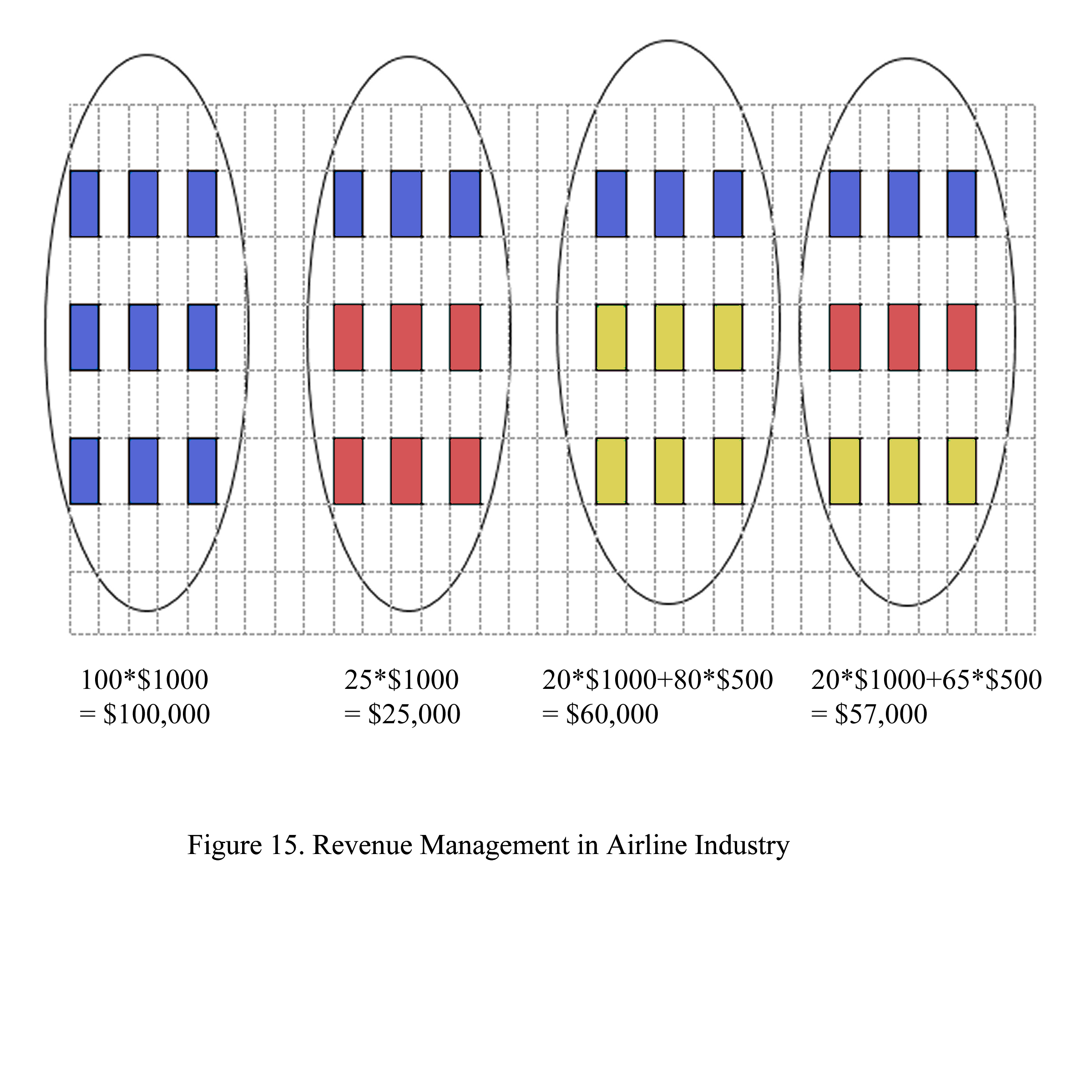
The rectangle bounded by these four points (p1, A, s1, and O) equals the price multiplied by the number of room nights sold. This is the hotel’s revenue including hotel cost (area 1) and hotel’s net profit (area 2). In Figure 12, area 1 of this graph corresponds to the hotel’s cost, which is obtained using the integral as follows:
Therefore, area 2 in the graph is the hotel’s net profit, or the area of the rectangle minus area 1.
3. Demand curve as utility cost
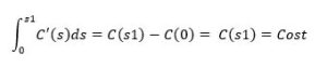
Demand is the quantity sold to the consumer by the producer. Hotel room demand is the number of room nights sold by the producer of the hotel. The demand is also measured by the maximum benefit of hotel guests during the period of staying at the hotel.
When consumers purchase z hotel room nights, the maximum benefit B(z) of the value of consumption u(z) is measured as follows:
B(z) = Total Value of Consumption – (Price * Quantity) = u(z) – p(z)
Where u(z) is a function describing the value of hotel room nights for all consumers.
Consumers will buy z1 hotel room nights when B(z1) is maximized; then B’(z1) = 0
The equation will be as follows:
B’(z1) = u’(z1) – p = 0 (Figure 13)
Consider the area of the rectangle labeled 3 above, which equals to the price p1 multiplied by the room nights sold z1. This is the total amount consumers pay for staying at the hotel.
The total area of 3 and 4 are obtained by using integration.
⨜0z1 u’(z)d(z) = u(z1) – u(0) = u(z1) = Total value of room nights sold.
Subtracting the value of the rectangle 3 from the integral from 0 to z1 we can find the benefit 4 to consumers.
4. Characteristics of business when applying Revenue Management
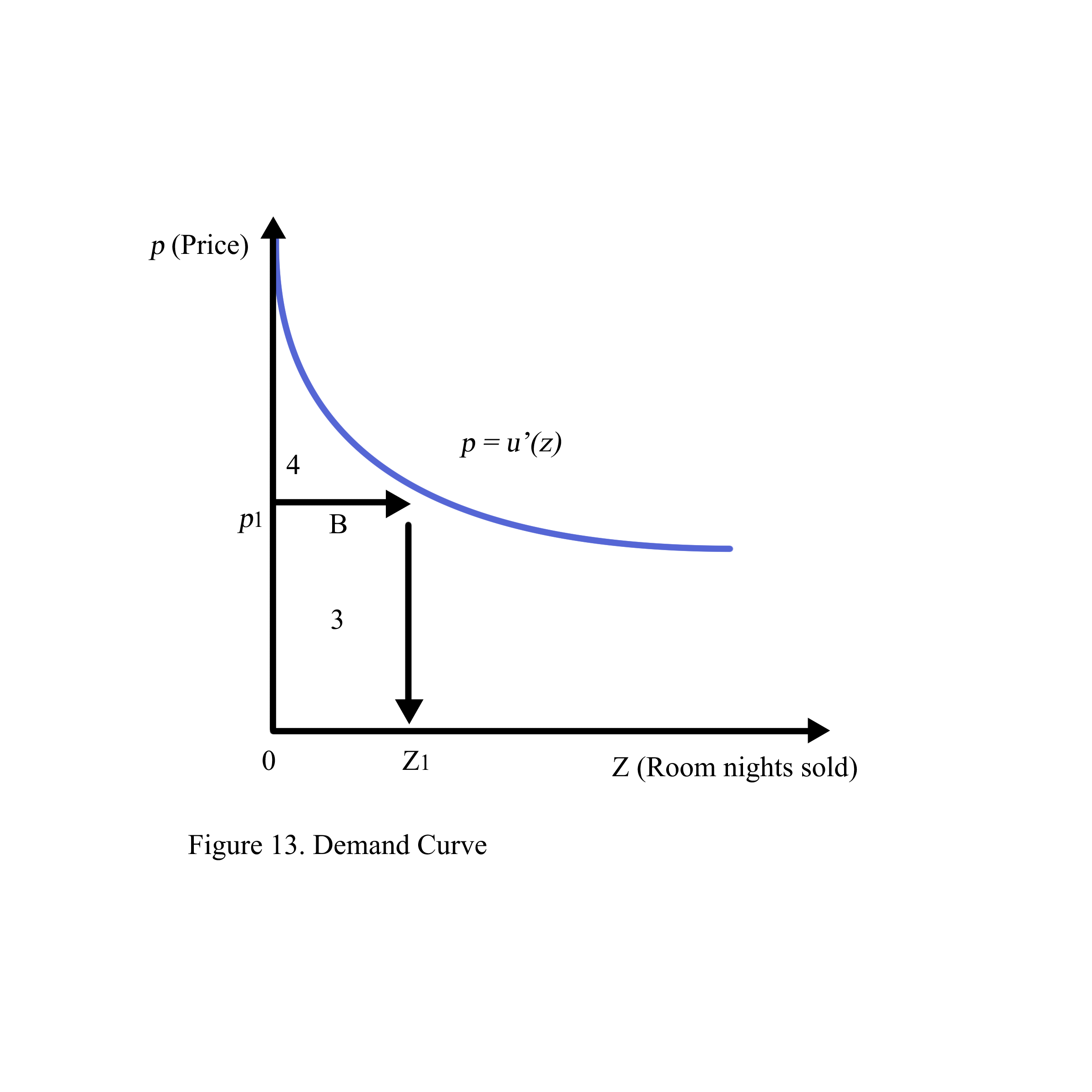
The revenue (blue rectangle CGHO) obtained from Supply (Cost Margin C’(x)) and Demand (U’(x)) is maximized due to zero marginal revenue R’(x) at point H. The profit (yellow rectangle BDFO) obtained from Cost Margin C’(x) and Revenue Margin R’(x) is maximized since the revenue margin R’(x) met the cost margin C’(x).
In sum, in order to measure revenue maximization and profit maximization, we need to have marginal revenue and marginal cost. The profit BDFO will be maximized at the price B when the marginal revenue R’ (x) equals the marginal cost C’ (x) at quantity F where demand (marginal benefit) is elastic (>1) and the revenue CGHO will be maximized at the price C when the marginal revenue R’ (x) equals zero at quantity H and demand (marginal benefit) is uni-elastic (=1).
Therefore, the producer starts his business with a loss (O) since the consumer receives most of the benefits (Ax0). The demand (marginal benefit) is inelastic (<1). Gradually, the producer gets the profit (CGO) from his maximized revenue (CGHO). At this time, the benefit AGC of the consumer is equal to the profit CGO of the producer. Then, the producer maximizes his profit BDFO at the elastic demand. Finally, if the producer increases the price from B to A, the profit will decrease till loss when quantity F moves to O quantity.
In conclusion, the producer only maximizes his profit when demand is elastic (Figure 14)
5. Optimal price between supply and demand
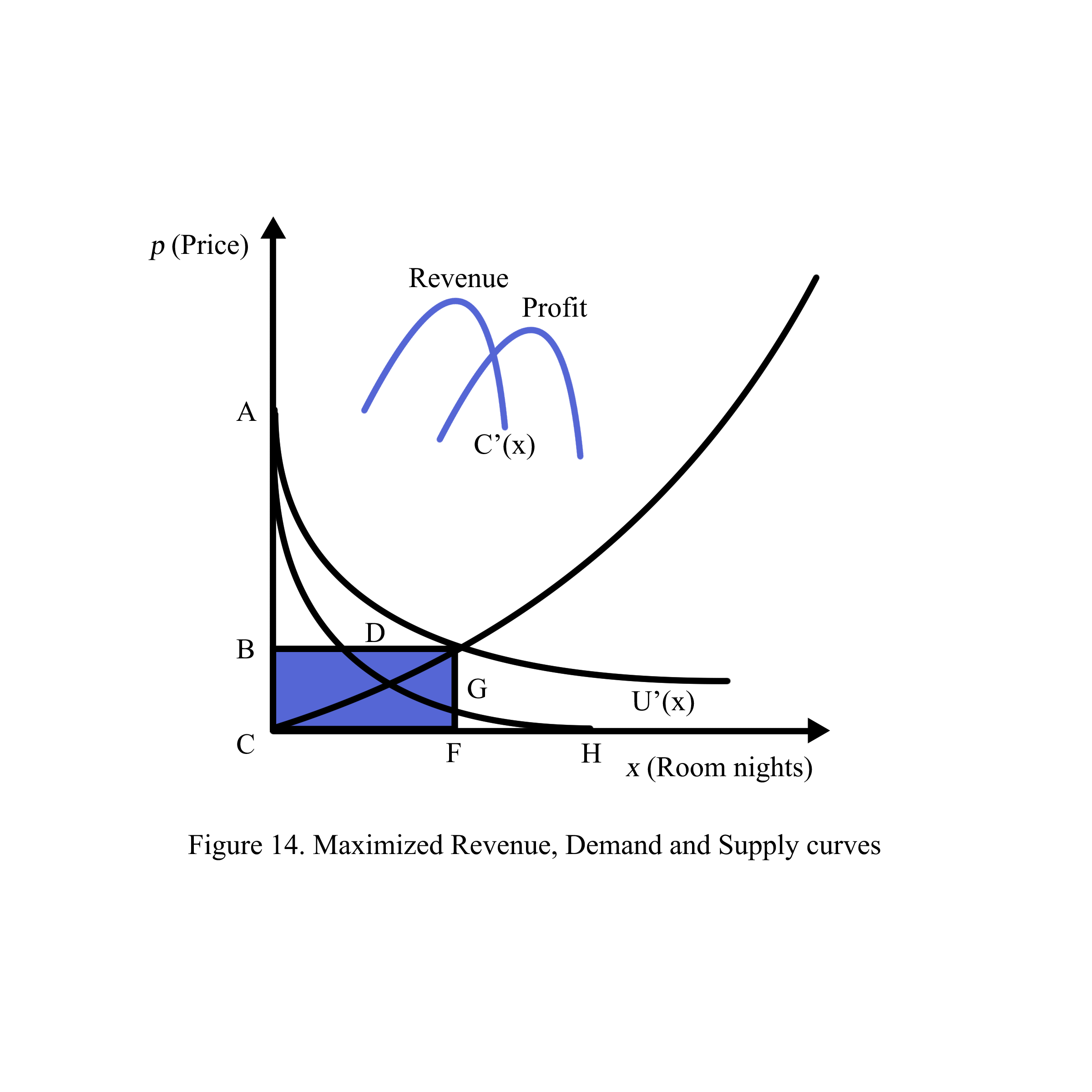
In the 1970s, major airlines maintained consistent ticket prices, even when seat availability became limited during peak seasons. However, as seat availability decreased, ticket prices began to rise accordingly. In 1978, American Airlines (AA) introduced the concept of Revenue Management. AA discovered that by adjusting the price of the same seat for different customers (referred to as Green or Blue) at different times (A, B, C, or D), they could maximize revenue, particularly as demand increased from the low season (B) to progressively higher-demand seasons (D, C, and A).
6. Industry applying Revenue Management
The industries that apply revenue management effectively often have 3 following characteristics: High fixed cost and low variable cost, fixed capacity and perishable products, and controllable demand.
(1) High Fixed Cost and low Variable cost
In the farming industry in small countries, the fixed cost is low so total cost will depend on high variable cost, which changes very often. In that case, when the marginal cost changes often lead to revenue margin change, revenue maximization is hard to forecast.
(2) Fixed capacity and perishable products
In the hotel industry, if we do not change the price for the perishable products, there will be a loss due to seasonal demand.
(3) Controllable demand.
The demand of the hotel can be affected by the pricing of the room.
Endnote
- Robert G. Cross, “Revenue Management: Hard-Core Tactics for Market Domination” (1997) ISBN 0307788989, 9780307788986. Revenue Management: Hard Core Tactics for Market Domination was a New York Times Business Best Seller and was published worldwide, in French, German, Japanese, Korean, Chinese, and Portuguese editions.
Key Terms
Hotel Revenue Management – The strategic process of using data analytics and forecasting to sell the right room to the right customer at the right price at the right time, maximizing a hotel’s revenue. It involves adjusting room rates and availability based on demand predictions, competitive analysis, and market conditions.
Hotel Revenue – The total income generated by a hotel from all its services, including room bookings, food and beverage sales, conference and event hosting, and additional amenities. This metric is crucial for assessing the financial health and performance of the hotel.
Hotel Demand – The total number of room nights sold for occupancy in a hotel or market. The level of desire for hotel rooms within a specific market or time frame. It fluctuates based on factors like seasonality, local events, economic conditions, and marketing efforts. Understanding demand helps in forecasting and pricing strategies.
Hotel Supply – The total number of room nights available for occupancy in a hotel or market. This includes all rooms that can be sold or rented out to guests. Supply, combined with demand, influences pricing and revenue strategies.
Hotel Average Daily Rate (ADR) – A key performance metric that calculates the average revenue earned per occupied room per day. It is obtained by dividing the total room revenue by the number of rooms sold, excluding complimentary rooms. ADR helps in assessing pricing strategies and revenue generation efficiency.
Hotel Revenue Per Available Room (RevPAR) – A critical indicator of a hotel’s financial performance, RevPAR measures the revenue earned per available room, regardless of whether the room is occupied. It is calculated by multiplying the ADR by the occupancy rate or by dividing total room revenue by the total number of available rooms. RevPAR helps in understanding how well a hotel is utilizing its available inventory.
Hotel Occupancy – The percentage of available rooms that are sold or occupied over a given period. It is calculated by dividing the number of occupied rooms by the total number of available rooms. Occupancy rates provide insights into a hotel’s capacity utilization and demand levels.
Review Questions
- Hotel A and hotel B has the same 100 rooms. What is the difference between two hotels A and B in terms of revenue at the end of the year?
- The cost of hotel sales is described in the function x3 with x is the number of room nights sold. What is the supply curve? How much are the cost and the profit of the hotel?
- The marginal utility of hotel guests is the function 3.4501e-0.323x and the optimal demand of the hotel guests is 1 room night. What is the benefit of the hotel guests?
- Measure the revenue, maximized revenue, demand function, price elasticity of demand (ChQ/ChP) from the Excel US Hotels 1990-2014 from Smith Travel Research
